Probably Approximately Correct Learning

Here, we familiarize ourselves with a formal learning model called Probably Approximately Correct learning (PAC Learning). This model relies on learning from observable examples, that is, the empirical, and hence is fallible to the limitations of all ERM learning paradigm, wherein the training sample can make or break the learner’s output.

The intuition

In simple speak, if you give the learner an upper bound on how incorrect your desired learning algorithm (or hypothesis) can be, the PAC learning model gives you the minimum number of examples that the learner should be trained on to achieve your desired error rate. We will thus focus on defining a notion of success of a learner, and the required sample complexity based on the bounds applied to this success. ⊕Recall that the learner is provided input of the form
(\(x_i, f(x_i)\)) where \(x_i\) is an instance from the input space \(\mathcal{X}\) distributed according to \(\mathcal{D}\), \(f\) is the true labelling function or classifier, and \(f(x_i)\) is the correct label of the instance. Based on the training sample comprised of \(m\) tuples of the form (\(x_i, f(x_i)\)) drawn in an i.i.d manner and labelled by \(f\), the learner has to successfully deduce oracle \(f\).

What do we actually mean by success in this context? We want to be able to say with a certain confidence that the learner’s output is an algorithm that makes predictions with a certain error rate. This error rate, or the probability that the learning algorithm produced by the learner fails at labelling instances from the input space, is represented in the term \(\epsilon\). This error rate is a proxy for accuracy, which is one component of what we mean by success. We assume that this error is due to the training sample available to the learner being a bad/misleading one, and/or the learner has overfit to it; consequently, the learner does not get enough information to help “deduce” \(f\).

Once we decide on the bounds of \(\epsilon\), it makes sense to say that any algorithm with an accuracy unacceptable by the bound (i.e \(< \epsilon\)) has failed. If we let \(\delta\) represent the probability of this failure, we have another knob to let us decide the bounds on how closely we want the learner’s output, let’s say \(h\), to approximate \(f\). Thus, we have confidence being represented by \(1 - \delta\).

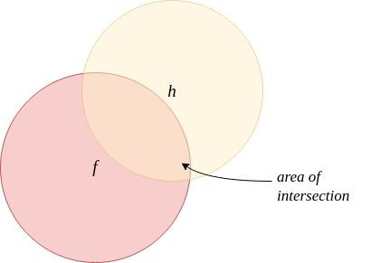
Let’s say we are dealing with a two-class classification problem, where the input space \(\mathcal{X} = \{0,1\}^n\) is \(n\) dimensional and binary in ⊕
If the total area is \(1\) and the area of intersection is \(a\), we need \(1 - a < \epsilon\). each, and the label space is \(\{0, 1\}\); we can express the true classifier as \(f : \{0,1\}^n \rightarrow \{0,1\}\). Let \(h\) be the hypothesis that the learner produces after training. Then, to qualify for PAC learnability, the learner must, with a probability of at least \(1-\delta\), find an \(h\) such that the symmetric difference between \(h\) and \(f\) is at most \(\epsilon\).

A formal definition

Let \(\mathcal{H}\) be a hypothesis class of boolean functions \(f : \{0,1\}^n \rightarrow \{0,1\}\). \(\mathcal{H}\) is PAC-learnable if there exists an algorithm \(\mathcal{L}\) such that for every \(f \in \mathcal{H}\), for any probability distribution \(\mathcal{D}\) over \(\mathcal{X}\), and arbitrary \(\epsilon\) and \(\delta\), if the realizability assumption holds, then the algorithm \(\mathcal{L}\) on input \(S \sim \mathcal{D}^m\), \(\epsilon, \delta\), outputs with confidence \(1-\delta\) over the training sample, the hypothesis \(h\) such that the generalization error \(L_{(\mathcal{D}, f)}(h) \leq \epsilon\).

Here, \(m \geq m_{\mathcal{H}}(\epsilon, \delta)\), where \(m_{\mathcal{H}}(\epsilon, \delta)\) is the function that gives the sample complexity, or the minimum number of examples the training set should have to give the above guarantee.

More about sample complexity

The sample complexity of learning a hypothesis class \(\mathcal{H}\) is given as \(m_{\mathcal{H}}(\epsilon, \delta): (0,1) \times (0,1) \rightarrow \mathbb{N}\), and as mentioned above, gives how many examples are required to guarantee a probably approximately correct solution. We lay stress on the observation that the sample complexity depends on the hypothesis class the learner is trying to learn, and can be fine tuned by the two free knobs \(\epsilon\) and \(\delta\). However, it doesn’t always make sense to use the full range of values that \(\epsilon\) can take; In the binary classification case that we are examining here, an \(\epsilon = 0.5\) implies that \(h\) is randomly labelling the instances. Therefore, the accuracy is usually bounded as \(0 \leq \epsilon <0.5\).

In the previous article on ERM, we already discussed the sample complexity of finite hypothesis classes, and showed that it depends on the log of the size of the hypothesis class. Additionally, we also note that if a hypothesis class is PAC learnable, then there are many functions \(m_\mathcal{H}\) that satisfy the requirements of the definition of PAC learning, but we want to know what the minimal integer that satisfies the requirements of PAC learning is. Therefore, any time we refer to the sample complexity function, it is implied that we mean the minimal function.