Gaussian Mixture Models and Expectation Maximization
Mixture models form a broad class of statistical models that essentially infer latent variables, i.e unobserved underlying patterns, from observable data. Such models are useful when a single distribution does not adequately capture the heterogeneity in data.
Mixture models are a probabilistically grounded way of performing soft clustering Soft vs. Hard Clustering:
Hard clustering is learning data that forms clusters which are well separated and do not overlap; datapoints either belong or do not belong to a given cluster.
Soft clustering is learning data that forms clusters that are not well separated and may overlap; datapoints have to be represented in terms of the strength of their association with different clusters, as opposed to the previous case with hard boundaries. , where each individual cluster is assumed to be a generative model, usually Gaussian or multinomial. As a whole, these models treat non-parametrized distributions over data as weighted mixtures of different known, parametrized distributions; the task of the learner then becomes inference of the parameters specifying the individual components of the distribution. Often, to simplify the learning task, it is assumed that the given distribution is a weighted mixture of Gaussians.
Expectation Maximization (EM)is one of the most popular algorithms utilized to learn from Gaussian Mixture Models (GMM). In general, the EM algorithm is useful to cluster the exponential family of distributions and is not limited to just Gaussian distributions. Let’s first understand what the problem at hand is, then at how the EM algorithm works.
The \(1-\)D Mixture Model
Consider a set of points in \(1-\)dimensional space.

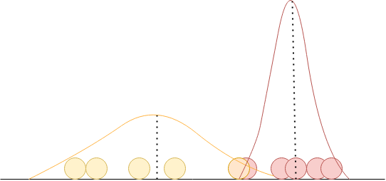
The ideal, labelled \(1-D\) dataset. Here, we colour in the datapoints to indicate the underlying distribution it is drawn from.

From a labelled dataset, it is easy to estimate the parameters of the underlying Gaussian components. Unfortunately, the learner does not have this luxury.

This is what the learner gets to see. Based on this, the learner is supposed to infer which points belong to which cluster.
Let’s say that the underlying process is based on coin flips, and depending on what face the coin lands on, a point is drawn from a corresponding Gaussian \(\mathcal{N}(\mu_i, \sigma_i)\) (where \(i\) can be either heads or tails). This process is repeated several times to form the training dataset given to the learner. Let’s say that the true distribution over these points looks somewhat like in the adjoining figure. If we are given insight into the process, a fully labelled dataset such as this makes estimating the parameters of the individual components a trivial task : All that has to be done is estimate the mean and variance for each category, namely, (\(\mu_{head}, \sigma_{head}\)) and (\(\mu_{tail}, \sigma_{tail}\)) separately. If the samples per category are fairly representative, the estimated values would be very close to the truth. Estimation can be done as follows:
\(\mu_i = \frac{\sum_j^{n_i}x_j}{n_i}\)
\(\sigma_i^2 = \frac{\sum_j^{n_i}(x_j - \mu_i)^2}{n_i}\)
where, \(x_j\) are the individual datapoints, \(n_i\) the number of points in cluster \(i\).
Unfortunately, the process occurs in a black box, and all that the learner has access to is the resultant dataset. So the learner not only has to estimate the parameters of the individual Gaussians in the mixture, it also has to be able reasonably pre-empt how many components (\(k\)) the mixture is composed of. Thus, when we don’t know the source of the datapoints, if we can infer the parameters of the Gaussians forming the mixture, we can guess whether the point is more likely to be part of the yellow Gaussian or the red one.
That is, if \(a\) represents the event that a datapoint has been drawn from the yellow Gaussian and \(b\), the event that a datapoint has been drawn from the red Gaussian, given a datapoint, we should after inferring the respective parameters be able to calculate the likelihood Since we know
\(P(x_i|a) = \frac{1}{\sqrt{2\pi\sigma_a^2}}\exp\bigg(-\frac{(x_i - \mu_a)^2}{2\sigma_a^2}\bigg)\)
\(P(x_i|b) = \frac{1}{\sqrt{2\pi\sigma_b^2}}\exp\bigg(-\frac{(x_i - \mu_b)^2}{2\sigma_b^2}\bigg)\)
and \(P(a)\), \(P(b)\).
using Bayes rule.
Herein lies the ultimate chicken and egg problem:
- To guess which distribution is the source of a given point, we need the parameters of the component Gaussians
- To estimate the parameters of the component Gaussians, we need to have access to the source of the datapoints.
The EM algorithm gives us an iterative mechanism by which we can infer the parameters of the component Gaussians, and thus find a way out of this loop.
EM Algorithm
Let \(k\) be the number of Gaussians in the mixture. We are still dealing with \(1-D\) Gaussian distributions; For higher dimensions, the algorithm is the same, with only very slight changes. In all cases, we assume symmetric, not skewed Gaussians as the components of the mixture.
Let \(G_i\) be the event that the datapoint was drawn from the Gaussian \(\mathcal{N}\)(\(\mu_i, \sigma_i\)). This is similar to what we represented using \(a\) and \(b\) earlier. Let \(x_j\) represent datapoints, where \(1 \leq j \leq m\).
Start with \(k\) randomly picked Gaussians with parameters (\(\mu_i, \sigma_i\)) for all \(i \in \mathbb{N}, 1 \leq i \leq k\)
Iterate until convergence:
- (E-step) For all datapoints in the training set, calculate the likelihood that it came from \(\mathcal{N}\)(\(\mu_i, \sigma_i\)). That is, calculate \(P(G_i|x_j)\). Note, this is calculated with respect to every Gaussian component, at every datapoint. These probabilities are used as weights \(w_{j_i}\) in the next step.
- (M-step) Adjust the parameters of each Gaussian by calculating them as follows:
Now, even if \(k=2\) in the relatively simpler \(1-D\) case, this algorithm takes a long time to converge if the sample complexity is high. In some scenarios, as the algorithm approaches convergence, it can get stuck in local optima and can take a very long time to converge. This algorithm is useful in practise but is not computationally efficient, and statistical analysis provies no bounds on the convergence rate.