Latent Variables and the Generative Model

Approaches to machine learning can be broadly classified as discriminative and generative. The discriminative approach aims to optimize accurate class prediction and does not make any assumptions about the data itself. The generative approach assumes a probabilistic model of the data. Any subset to be trained on is assumed to be sampled according to an underlying distribution with a parametric form, over the data that forms the input space. The task then becomes learning, or inferring, the parameters that fully describe the data distribution of the given parametric form. This task is dubbed parametric density estimation.

Latent variable models

Let’s say that you are building a probabilistic language model of news articles. Each article \(x\) is ⊕
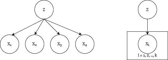
Graphical representation of a latent variable model, also known as a topic model based on a certain topic \(z\) – such as sports, education, op-ed, and so on. The idea here is that the language model \(p\) assigns probabilities to strings of words \(x_1, x_2, ..., x_n\), and we can sample from the model by generating different kinds of sentences, based on the topic \(z\) of interest. Essentially, you draw an article out of a bag of words that correspond to a particular topic.

Now, given an article, i.e, the observable variable, we want to be able to infer the topic, i.e, the latent variable. If successful, the classifier that results would be a Bayes optimal classifier. This model would allow the machine to now learn a separate distribution \(p(x\mid z)\) for each topic, rather than trying to model everything with one distribution over the observable data.

Why use LVMs at all?

Latent variable models allow us to leverage prior knowledge when defining a model. The example above illustrates this. We know that our set of articles is a mixture of distributions (one per topic) and latent variable models allow us to capture this structure. This imbues the model with higher expressive power than anything we could have obtained by building a model over just the observable components of the data.

Note here that latent variable models are often represented by Bayesian networks or directed graphical models (as shown the first diagram), which insinuate a causal relationship between the observable and latent variables. But this is a trap. While the representation encodes dependency, it does not necessarily represent a causal relationship.

Learning LVMs

Very briefly, our goal is to fit the marginal distribution \(p(x)\) over the observable variables in our dataset. We calculate the marginal by summing out the joint distribution over the latent variable model, represented by \(p(x, z)\). Ideally, we would then want to maximize the likelihood, i.e, the marginal we just calculated. The loss minimized here would be the Kullback-Liebler divergence. But it’s not as easy to do in practise. Here’s why:

Now, doing this for every observable variable in the dataset \(D\), we can write \(\log p(D) = \sum_{x \in D}\log p(x) = \sum_{x \in D}\log \bigg(\sum_zp(x \mid z)p(z)\bigg)\)

Maximizing over this objective is more difficult than the regular log-likelihood maximization because of the summation inside the log – you cannot decompose \(p(x)\) into a sum of log-factors, so even if the model is a directed model, there is no simple closed form expression for the parameters. Moreover, the marginal for a given datapoint \(x\) can be seen as a weighted mixture of the different distributions that it is composed of. That is, the marginal is a sum of the individual distibutions \(p(x \mid z)\) weighted by \(p(z)\). Assuming that the marginal belongs to the exponential family, the log of such a mixture distribution is not concave or convex, and we must use specialized methods for non-convex optimization.